The major goal for the 2020 micromouse was to do curves without stopping. This would require deviating from last year's software architecture in a few ways. The mouse could no longer assume that it was traveling down the center of the cells, nor that it would stop at the end of every move.

There were also a few things I wanted to change that are not necessarily related to curves. For one, there were a lot of control loops going on: up to six at a time. Many of these were leftover from the quick development process, and made tuning fairly difficult. There were also a lot of nested control structures, and references to them got passed around a lot. This made everything tightly coupled, and significantly changing something would require a fair bit of work. This lead to a few secondary goals: to avoid nesting and tight coupling, and avoiding extra control loops. To avoid nesting and tight coupling between control structures and modules, each control structure would operate independently of each other, and communicate through simple types passed as function arguments and return values.

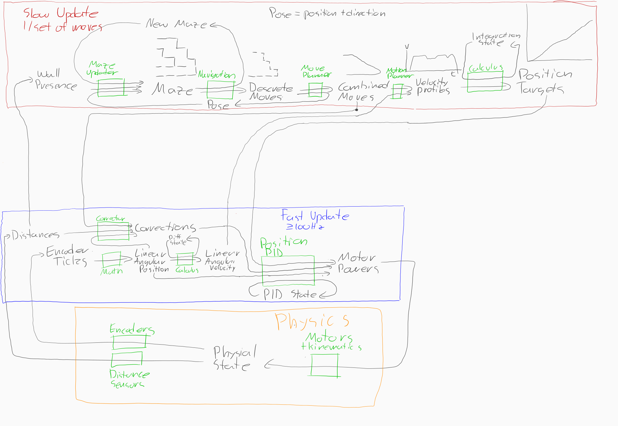
The first step was to figure out a general structure and data flow. Because the mouse would no longer always be traveling straight down the center of a cell, it would need to know where it is and what direction it is facing relative to the maze as a whole. It would also need to know what path it is trying to follow, with no interruptions. Here is what I came up with:

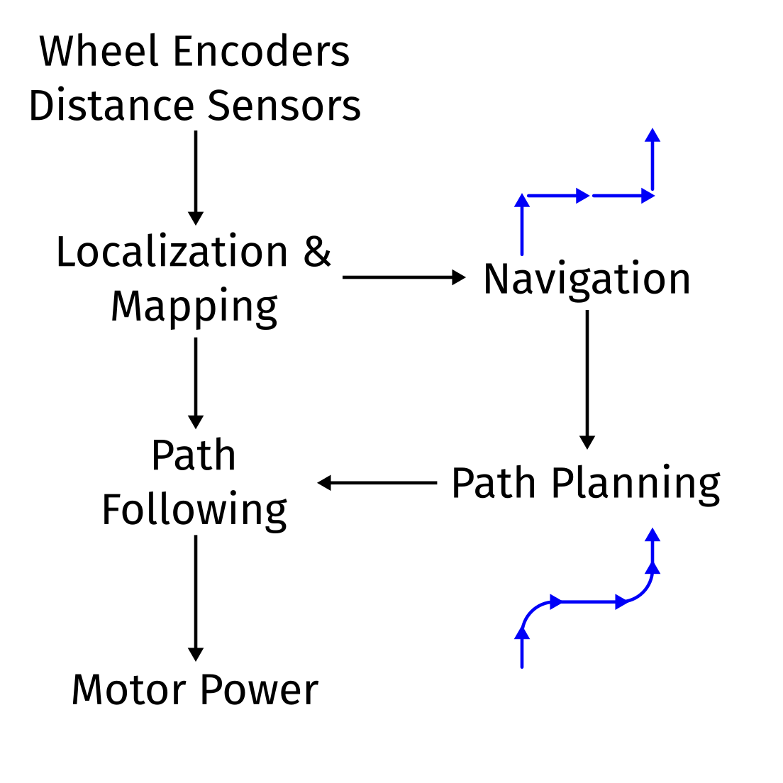
There are two main paths here. The left is the fast path. It does all the motion control loops that need to happen in real time. The right is the slow path. It does any higher-level navigation and planning functions, and will only run when the fast path runs out of paths to follow.

The fast path

The fast path is in charge of reading the sensors, figuring out where the mouse is and what the maze is, and controlling the motors to follow a path. It is split into two main parts: localization and mapping, and path following.

Localization

Localization takes in the sensor values, both the encoders on the wheels and the distance sensors for the walls. There are a few data types associated with localization: Direction, Vector, and Orientation, defined below.

/// a 2d vector
pub struct Vector {
    pub x: f32,
    pub y: f32,
}

/// a direction wrapped to 0 - 2pi
pub struct Direction(f32);

/// the combination of position and direction
pub struct Orientation {
    pub position: Vector,
    pub direction: Direction,
}

These should be mostly self-explanatory. the Direction type is a little special, though. since Direction is an angle in radians, it only makes sense for it to be between 0 and 2π. To enforce this, the internal f32 field is not public, and the only interaction can happen through methods and trait implementations on Direction. This is primarily done with the From and Into traits:

impl From<f32> for Direction {
    fn from(other: f32) -> Direction {
        Direction((other + 2.0 * PI) % (2.0 * PI))
    }
}

impl From<Direction> for f32 {
    fn from(other: Direction) -> f32 {
        other.0
    }
}

Localizing starts with the encoders. Given the last known orientation and the change in encoders, it can figure out the current orientation:

impl Orientation {
    /// Update the orientation with new encoder data. The encoders will be converted from ticks to
    /// mm and radians using the MechanicalConfig provided.
    pub fn update_from_encoders(
        self,
        config: &MechanicalConfig,
        delta_left: i32,
        delta_right: i32,
    ) -> Orientation {
        // The change in linear (forward/backward) movement, converted to mm
        let delta_linear = config.ticks_to_mm((delta_right + delta_left) as f32 / 2.0);

        // The change in angular (turning) movement, converted to radians
        let delta_angular = config.ticks_to_rads((delta_right - delta_left) as f32 / 2.0);

        // Assume that the direction traveled from the last position to this one is halfway
        // between the last direction and the current direction
        let mid_dir = f32::from(self.direction) + delta_angular / 2.0;

        // Now that we have an angle and a hypotenuse, we can use trig to find the change
        // in x and change in y
        Orientation {
            position: Vector {
                x: self.position.x + delta_linear * F32Ext::cos(mid_dir),
                y: self.position.y + delta_linear * F32Ext::sin(mid_dir),
            },
            direction: self.direction + Direction::from(delta_angular),
        }
    }

    //...
}

This works out pretty well, but it is susceptible to drift over time. If the mechanical parameters do not match real life perfectly, or if the wheels slip, the calculated orientation will slowly get further away from reality. Although this error may be small at first, it could be off by quite a bit after a few minutes.

To help account for this, the orientation gets adjusted based on what the distance sensors are reading. It turns out that there is actually a lot of information that you can get from the three distances, assuming you know what walls you are looking at. Even better, the most common situation of having the two side walls parallel and the front wall perpendicular to the mouse will fully constrain both the position and the direction of the mouse relative to those walls. This was my first attempt at using the distance sensors. I implemented the math for this and a few other cases, but there were issues. The first problem is that you need to know what you are looking at. While this is calculable if the maze is known, it becomes very sensitive to errors in your estimated orientation. If you are looking right at the edge of a wall, it is easy to actually be looking just next to it, at a wall several cells down a corridor. The second issue is sensor noise. The distance sensors on the mouse can vary by a few millimeters, causing the calculated orientation to jump around. This can cause all sorts of issues when the path following tries to get the mouse to go straight, but it keeps moving in unexpected ways. I initially tried to make this work in a few ways. If the expected and actual distances read are too different, you probably are not looking at the right wall. The sensor readings can be filtered to minimize the jumping. There were a host of other things I tried as well. However, none of these could fix the underlying issues, and took away a lot of the benifits of this approach.

I decided to throw it all out and try again. A lot of the issues came from the complexity of trying to work everywhere, and working around the cases when it didn't work. If I could come up with something that worked good enough most of the time, the funny edge cases could fall back to the encoders. It turns out the most of the time, the mouse is traveling straight down the center of the cell. This case also happens to have the simplest math. To take advantage of this, I had the mouse only try to use the sensors if the path it was following was pointed roughly straight through the cell. This ended up working pretty well.

Mapping

Mapping is supposed to take in the current orientation and the distance sensor readings, and map out the maze as the mouse travels. This could then be used by the navigation algorithm. Since the algorithms we had did not actually use the full maze, and a lack of time, the mapping ended up just giving whether the mouse could move forward, left, and/or right.

Path Following

Now for the exciting part. The path following module needs to take in the mouse's current location, and adjust the motor powers to follow a path.

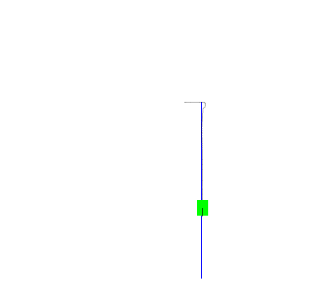
The first attempt was to use CSP, or cyclic synchronous position control. This is where each motor has a velocity and position PID loop, which gets streamed a set of position targets. These targets would be generated ahead of time, based on the path to follow. Here is a rough diagram:

However, I could see a few problems. The first was move corrections. Because the position targets are calculated ahead of time, it becomes difficult to use the current position to correct them. The other issue is that CSP attempts to strongly control both linear and angular velocity and position, it would seem that we really only care about angular velocity. By controlling linear as well, we need to account for acceleration and deceleration, complicating the process. Not to mention that at least 4 PID loops would be needed.

But what if we only controlled the angular velocity? Then, we might be able to get away with only one PID loop, we don't need to care what the actual linear velocity is, and adjusting for new orientations is relatively easy. But what would be the error signal? Well, we are trying to follow a path, which means the mouse wants to be on the path. Also, being further away from the path means the mouse wants to turn more. It would make sense to use the distance away from the path as the error for the PID controller. Luckily, this is easy to calculate for a path made up of lines and arcs, so I wrote a simulation and tried it out. Unfortunately, it didn't go too well:

With some tuning, it got a lot better:

However, things were not all fine and dandy. After running on a closed loop for a while, the mouse would become unstable. Even after following perfectly for a while, the mouse would start to oscillate around the path. Once the mouse makes it to the center, it keeps going in the direction it was going, not along the path. This causes it to miss shoot the path, and doesn't start to turn back until it gets far enough away. It would then turn around, but keep turning, since the angular velocity won't go down until it gets sufficiently close to the path. Once it gets far enough away, it never makes it back. It just keeps circling. This can be mitigated with a high D term. As the mouse gets closer faster, the D will increase, pushing it back out, until it comes smoothly back to the path. However, this high D will also amplify any noise in the system, and can become unstable quickly. So, it would seem that the system is unstable because there is an extra integration in the feedback loop. Because of the geometry, keeping the angular position constant will cause the distance integrate once. Keeping the angular velocity constant causes the angular position to change at a constant rate, integrating a second time.

It would seem that controlling angular position would be a better choice than angular velocity. But what angular position should it target? Well, we want the mouse to travel in the general direction of the path, so the path direction is a good start. But we also want the mouse to make it's way back toward the path, but smoothly approach the path rather than go directly for it. Thus, the target angular direction needs to depend on the distance from the path as well. An easy way to do this would be to multiply the distance from the path by a constant factor, then add the direction of the path.

With this, things worked a bit better:

This could run all day with no issues, with only the slight cost of adding another tuning parameter.

While things seemed pretty good in the simulator, there were issues running this on a mouse. The first signs of trouble showed when I tried to run the mouse in a loop for a while. After not too long, the direction would start to be off, and the whole loop would be angled. At first, I thought that I had measured the distance between the wheels incorrectly, so I remeasured, and it seemed right. I started to try and adjust the distance in the config to to fudge it to work, but I could never quite get it right. Even when it was close, it was a a bit different from the real number. This lead me to think that there could be slippage on the turns, so I set out to try and tune it to be smoother. While tuning for a mouse on the bench, it needed really high D values to go around the curves without taking too long to turn back on course. This looked suspicious, so I took a look at the graphs of motor power. At the start of each turn, it would need to spike the motor power all the way to the extremes to get it to start turning, and spike to the opposite extremes to get it to stop turning. In the simulator, it just started turning immediately since inertia was not simulated. However, the real mice do have inertia. This spike, no matter how big, could not get the mouse to turn fast enough. It also seemed that this spike caused the wheels to slip right as the turn was starting, which explained the direction errors. Even in the simulator, it looked like a high enough D was needed to closely follow the path that it would amplify the floating point errors when traveling straight, which led to strange behaviors.

I had been using normal, circular arcs for the curves. Now that I thought about it, going from a straight to an arc would require the wheels to change velocity instantaneously. Going straight required a fixed speed, and doing an arc requires a fixed, but different speed. The wheels could not change speed fast enough. I would need to find a different way to do the curves, one that would gradually ease into the turn.

I started looking at Bezier curves, since they seemed to be smoother that just an arc. Bezier curves are described by a number of control points. One at each end, then some number of them in the middle. Beziers are characterized by the number of control points. A curve with 3 control points is a 2nd order Bezier, 4 control points is a 3rd order Bezier, and so on. Mathematically, they are parametric functions described by a polynomial.

In researching them, I came across this site: https://pomax.github.io/bezierinfo/. The site explains Bezier curves, the math behind them, and operations that can be performed on them. In the midst of all this, the site mentions the "Curvature of a curve", which stuck out to me. It goes on to say:

In fact, it stays easy because we can also compute the associated "radius of curvature", which gives us the implicit circle that "fits" the curve's curvature at any point, using what is possibly the simplest relation in this entire primer: R(t) = 1/k(t). So that's a rather convenient fact to know, too.

Hmm, so the curvature is the inverse of the radius at a given point. This means that a straight line has a curvature of zero, and an arc has a constant, non-zero curvature. If I could get the Bezier curve to start at zero curvature, gradually increase to a peak curvature, then gradually decrease back to zero, we could be in business. I did a little searching to see if anyone else had used Bezier curves for robot path planning, and came across this paper: https://www.hindawi.com/journals/jat/2018/6060924/. This describes using Bezier curves for autonomous car path planning. In it, this paragraph appears:

The previous equation explicitly shows that if the three starting points in a curve are colinear, generated Bézier curve will have zero curvature at its starting point (k(t = 0) = 0); this can be extended to the three ending points due to symmetry. This property is useful for designing the intersections and lane changes, and for the entrance and exit part of the roundabout.

If there are three control points in a row at either end, then the curvature at that end is zero. Perfect! This is exactly what we need to match with a straight line. I started with 3rd order curves, because they are the minimum needed to get 3 points in a row from both ends, if you put the two middle control points on top of each other.

It turns out that curvature also has physical meaning: radians of turning per mm of travel. If you're driving a car, this is how much you have the steering wheel turned. If you're stopped, it doesn't matter how much the wheel is turned. But as soon as you start moving, the car will follow the wheel. You can speed up and slow down without changing where you are going, and if you turn the wheel, you don't necessarily need to change speed. However, as any new driver quickly figures out, you can't just slam the wheel to one side. You also need to watch you're speed when going around a sharp turn. These constraints apply to the mouse as well: The peak curvature cannot be too high, and the curvature can only change so fast. By putting 3 points in a row, we are ensuring that the wheel starts in the center.

Since I couldn't find any good Rust Bezier curve libraries for embedded, I wrote it myself:

pub struct Bezier3 {
    pub start: Vector,
    pub ctrl0: Vector,
    pub ctrl1: Vector,
    pub end: Vector,
}

impl Curve for Bezier3 {
    type Derivative = Bezier2;

    /// Evaluate the curve at `t`
    fn at(&self, t: f32) -> Vector {
        Vector {
            x: self.start.x * (1.0 - t) * (1.0 - t) * (1.0 - t)
                + 3.0 * self.ctrl0.x * (1.0 - t) * (1.0 - t) * t
                + 3.0 * self.ctrl1.x * (1.0 - t) * t * t
                + self.end.x * t * t * t,

            y: self.start.y * (1.0 - t) * (1.0 - t) * (1.0 - t)
                + 3.0 * self.ctrl0.y * (1.0 - t) * (1.0 - t) * t
                + 3.0 * self.ctrl1.y * (1.0 - t) * t * t
                + self.end.y * t * t * t,
        }
    }

    fn derivative(&self) -> Self::Derivative {
        Bezier2 {
            start: 3.0 * (self.ctrl0 - self.start),
            ctrl0: 3.0 * (self.ctrl1 - self.ctrl0),
            end: 3.0 * (self.end - self.ctrl1),
        }
    }
}

Short and sweet. The Bezier itself is just the four control points. The Curve trait defines operations that could apply to any curve, Bezier or not. This make it easy to switch in different types of curves to the path following algorithm. It also includes default methods for calculating the curvature and finding the closest point on the curve, so they don't need to be reimplemented every time. Of course, curves like Arc or Line just reimplement these with constants, so there is no extra computation.

This means that instead of trying to control the mouse's angular velocity, we can control it's curvature. We can turn the smoothly. This has the added benefit that if the mouse's (uncontrolled) linear velocity changes, it will not change the curve that it is doing. At first, I to directly control the curvature with a PID loop. It targeted the curvature from the path, and ultimately output an angular power for the motors. This worked pretty well, but it had a few issues. For one, there was no adjustment to try and get back on the path, but that can be implemented later. It also would not easily account for differences between the motors. It would be up to the I portion of the PID to settle that. It also had some hairy math to calculate the current curvature from the encoders, and to make the curvature back into motor powers. To make some of this a little easier, I changed it to do a PID loop on velocity for each of the wheels, and calculate the target velocity for each wheel based on the target curvature and linear velocity. This fixed the motor differences problem, and made the math a lot simpler.

To the the mouse back on the path, I used a similar approach to when it was controlling angular velocity. It would calculate a target direction, then use that to find a curvature. At first, it would try to calculate this curvature based on geometry, given the current linear velocity and the time between steps, to get a curvature that would result in pointing the right direction the next time the function was called again. However, this did not always work well with physics, since the mouse would generally not end up at the target angle. To fix this, I added a third PID loop. This one would try to calculate an adjustment curvature based on the target angle. This adjustment curvature is then added to the curvature of the path to get the final curvature.

Overall, this worked pretty well:

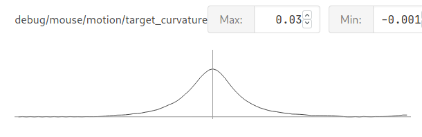
Even in the simulation, the mouse was able to follow much closer than with the arcs. The target curvature graphed from the simulation is also quite smooth, peaking at about 0.02 rads/mm. In real life, this also worked. The mouse follows the path around corners:

Not perfect, but pretty good.

One thing I noticed, however, was that the mouse would turn fairly sharply at the middle of the curve. This indicated that the peak curvature was too high. However, the 3rd order Bezier curves only have one possibility if we want zero curvature at the ends, 90 degree turns, and keep the endpoints from going too far out. I would need a higher order curve to have some adjustment. I took a hint from the paper linked above, and decided to try 5th order curves. These would have a total of 6 control points, which allows 3 in a row at each end. The distance between these points can be adjusted to changed the curvature along the curve. In implemented this in much the same way as the 3rd order curve, and it was pretty easy to switch out.

But what distance should the points be adjusted to? Putting the points closer to the center would make the peak higher, but the lead in smoother. Putting them towards the ends would lower the peak, but make the lead in more sudden. To visualize this, I turned to GeoGebra. It allows graphing, solving, and various other math things for just about anything.

Here is a 5th order Bezier curver with control points A, B, C, D, and E:

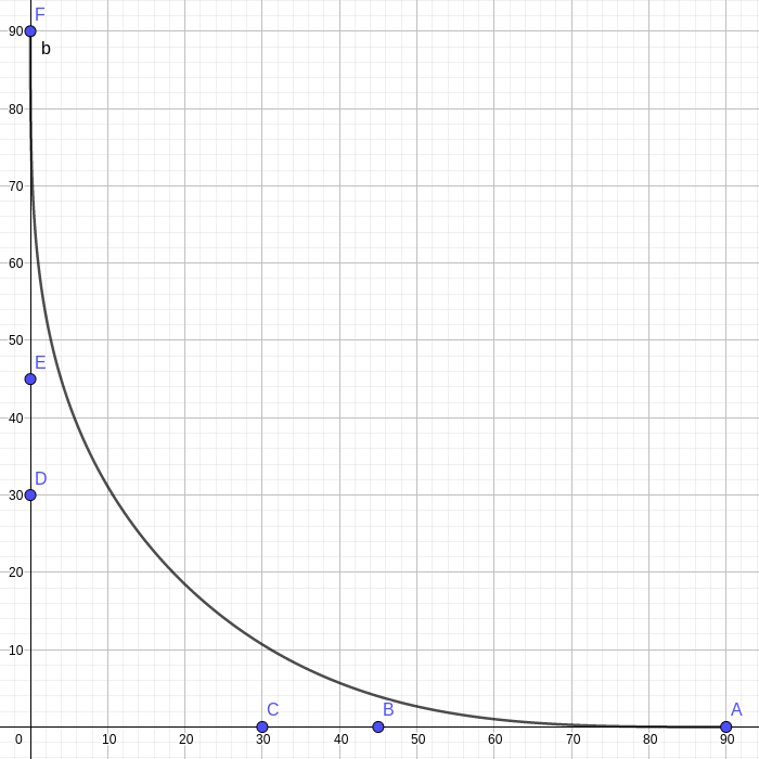
Here is the same Bezier, but in 3d, and curvature along the curve in the 3rd dimension, in red:

(Note the units on the axis. They match a real curve for a maze)

Using this, I could adjust the control points and see how the curvature responds. After a bit of twiddling and trying things on the mouse, I came up with something that worked. For a given distance r from the origin to the endpoints, putting the points at r/2 and r/3 worked pretty well.

With these 5th order Beziers and some tuning, the mouse was running pretty well. Now, it needed to use the distance sensors to avoid hitting walls, and then we might be ready for some maze navigation!